(ε, δ)-definition of limit
In calculus, the (ε, δ)-definition of limit ("epsilon-delta definition of limit") is a formalization of the notion of limit. It was given by Bernard Bolzano, in 1817, and in a less precise form by Augustin-Louis Cauchy.[1][2]
Contents |
History
Isaac Newton was aware, in the context of the derivative concept, that the limit of the ratio of evanescent quantities was not itself a ratio, and at points explained limits in terms similar to the delta-epsilon definition.[3] Augustin-Louis Cauchy gave a definition of limit in terms of a more primitive notion he called a variable quantity. He never gave an epsilon-delta definition of limit. Cauchy's foundational approach exploits infinitesimals in a fundamental and systematic way, as he mentions in the introduction to the Cours d'Analyse. Some of Cauchy's proofs contain indications of the epsilon, delta method. Whether or not his foundational approach can be considered a harbinger of Weierstrass's is a subject of scholarly dispute. Grabiner feels that it is, while Schubring (2005) disagrees.[1]
Informal statement
Let ƒ be a function. To say that
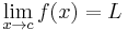
means that ƒ(x) can be made as close as desired to L by making the independent variable x close enough, but not equal, to the value c.
How close is "close enough to c" depends on how close one wants to make ƒ(x) to L. It also of course depends on which function ƒ is and on which number c is. The positive number ε (epsilon) is how close one wants to make ƒ(x) to L; one wants the distance to be less than ε. The positive number δ is how close one will make x to c; if the distance from x to c is less than δ (but not zero), then the distance from ƒ(x) to L will be less than ε. Thus δ depends on ε. The limit statement means that no matter how small ε is made, δ can be made small enough.
The letters ε and δ can be understood as "error" and "distance", and in fact Cauchy used ε as an abbreviation for "error" in some of his work.[1] In these terms, the error (ε) in the measurement of the value at the limit can be made as small as desired by reducing the distance (δ) to the limit point.
This definition also works for functions with more than one input value. In those cases, δ can be understood as the radius of a circle or sphere or higher-dimensional analogy, in the domain of the function and centered at the point where the existence of a limit is being proven, for which every point inside produces a function value less than ε from the value of the function at the limit point.
Precise statement
The (ε, δ)-definition of the limit of a function is as follows:
Let ƒ be a function defined on an open interval containing c (except possibly at c) and let L be a real number. Then the formula
means
- for each real ε > 0 there exists a real δ > 0 such that for all x with 0 < |x − c| < δ, we have |ƒ(x) − L| < ε,
or, symbolically,

The real inequalities exploited in the above definition were pioneered by Bolzano and Cauchy and formalized by Weierstrass.
Continuity
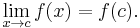
A function ƒ is said to be continuous at c if it is both defined at c and its value at c equals the limit of f as x approaches c:
If the condition 0 < |x − c| is left out of the definition of limit, then requiring ƒ(x) to have a limit at c would be the same as requiring ƒ(x) to be continuous at c.
f is said to be continuous on an interval I if it is continuous at every point c of I.
Comparison with infinitesimal definition
Keisler proved that a hyperreal definition of limit reduces the quantifier complexity by two quantifiers.[4] Namely, f(x) converges to a limit L as x tends to a if and only if for every infinitesimal e, the value f(x+e) is infinitely close to L (see microcontinuity for a related definition of continuity). While infinitesimal calculus textbooks based on Robinson's approach provide definitions of continuity, derivative, and integral at all real points in terms of infinitesimals to the exclusion of epsilon, delta methods, Hrbacek writes that the definitions of continuity, derivative, and integration in non-standard analysis implicitly must be grounded in the ε-δ method in order to cover also non-standard values of the input. Thus, Hrbacek argues, the hope that non-standard calculus could be done without ε-δ methods can not be realized in full.[5]
See also
Notes
- ^ a b c Grabiner, Judith V. (March 1983), "Who Gave You the Epsilon? Cauchy and the Origins of Rigorous Calculus", The American Mathematical Monthly (Mathematical Association of America) 90 (3): 185–194, doi:10.2307/2975545, JSTOR 2975545, archived from the original on 2009-05-03, http://www.webcitation.org/5gVUmZmxc, retrieved 2009-05-01
- ^ Cauchy, A.-L. (1823), "Septième Leçon - Valeurs de quelques expressions qui se présentent sous les formes indéterminées
 Relation qui existe entre le rapport aux différences finies et la fonction dérivée", Résumé des leçons données à l’école royale polytechnique sur le calcul infinitésimal, Paris, archived from the original on 2009-05-03, http://gallica.bnf.fr/ark:/12148/bpt6k90196z/f45n5.capture, retrieved 2009-05-01, p. 44.. Accessed 2009-05-01.
 - ^ Pourciau, B. (2001), "Newton and the Notion of Limit", Historia Mathematica 28 (1)
- ^ Keisler, H. Jerome (2008), "Quantifiers in limits", Andrzej Mostowski and foundational studies, IOS, Amsterdam, pp. 151–170
- ^ Hrbacek, K. (2007), "Stratified Analysis?", in Van Den Berg, I.; Neves, V., The Strength of Nonstandard Analysis, Springer
Bibliography
- Schubring, Gert (2005), Conflicts Between Generalization, Rigor, and Intuition: Number Concepts Underlying the Development of Analysis in 17th–19th Century France and Germany, Springer, ISBN 0387228365